Understanding WaveNet architecture

WaveNet is deep autoregressive, generative model, which takes raw audio as inputand produces human-like sound.This has brought new dynamics in speech synthesis. WaveNet is combines two ideas, which are Wavelet transform and Neural networks. As given in original paper, it was stated that speech of human in raw form is generally represented as a sequence of 16 bit and it produces total of \(2^{16}\) (65536) quantization values. This quantization values has to be processed through softmax, as 65536 neurons would be required. Hence making this computationally expensive. The need for reducing the sequence to 8 bits was required. This is done using \(\mu\)-law transformation, which is represented as \(F(x) = sign(x) \frac{ln(1+ \mu \lvert x \rvert)}{(1+\mu)}\), -1 ≤ x ≤ 1, where \(\mu\) takes value from 0 to 255 and x denotes input samples and then quantize to 256 values. The first step in an audio preprocessing step requires converting input waveform to quantized values, which has fixed integer range. The integer amplitudes are then one-hot encoded. These one-hot encoded samples are passed through causal convolution.

Causal Convolution Layer

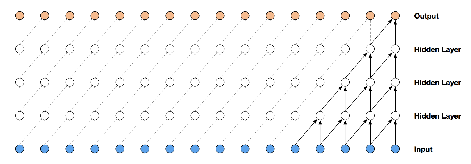
Causal system referred in signal and system, as the system which depends on the past and current inputs but not on future inputs. It is practically possible to implement causal system. In WaveNet the current acoustic intensity of the neural network is produced at time step t only depends on data before t. This layer is the main part of architecture, as it signifies autoregressive property of WaveNet and also maintains ordering of samples.

For training of 1 output sample, 5 input samples are used. Receptive field of this network is 5. The following equation is used for generation of new samples by predicting probability of next samples, given the probabilities of previous and current samples. \[ p(x) = \prod_{n=1}^{N} p(x_{N} \mid x_{1}, x_{2} \dots, x_{N-1}), \] where samples are denoted as \(x = (x_{1}, x_{2} \dots, x_{N})\), \(p(.)\) is the probability. Problem with causal convolution is that they require many layers, or large filters to increase the receptive field.

Dilated Convolution Layer

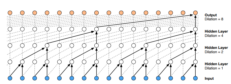
Dilated Convolution also referred as Convolution with holes or a-trous Convolution. In standard convolution (dilation =1), kernel varies linearly. It is equivalent to a convolution with a larger filter, wherein the original convolution is filled with zeros to increase the receptive field of the network. Stacked dilated convolutions enable networks to have very large receptive fields with just a few layers, while preserving the input resolution throughout the network as well as computational efficiency. For training of 1 sample, total of 16 inputs are required, as compared to 5 in causal convolution.

Each \(1, 2, 4, \dots, 512\) block has receptive field of size 1024, and can be seen as a more efficient and discriminative (non-linear) counterpart of a 1×1024 convolution. The model gets struck where the input is nearly silent, as the model is confused about the next samples to be generated.

Gated Activation Units

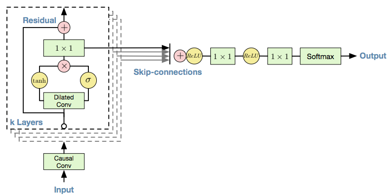
The purpose of using gated activation units is to model complex operations. The gated activation units is represented by the following equation: \[ z=\tanh(W_{f,k} \ast x).\sigma(W_{g,k} \ast x) \] where \(\ast\) is a convolution operator, . is an element wise multiplication operator,\(\sigma(.)\) is the sigmoid activation function, k is the layer index and \(W_{f}\) , and \(W_{g}\) , are weight matrix of filters and gate respectively.

Residual block and Skip Connections

The use of residual block and skip channels is inspired from PixelCNN architecture for images.Both residual and parameterized skip connections are used throughout the network, to speed up convergence and enable training of much deeper models.

Global and Local Conditioning

When WaveNet model is conditioned on auxillary input features (linguistic feature or acoustic feature), denoted by h(latent representation of features), it is represented as \(p(x \mid h)\) \[ p(x \mid h) = \prod_{n=1}^{N} p(x_{N} \mid x_{1}, x_{2} \dots, x_{N-1},h) \]. By conditioning the model on other input variables, we can guide WaveNet’s generation to produce audio with the required characteristics. WaveNet model is conditioned based on the nature of input in 2 ways : a) Global Conditioning, b) Local Conditioning. Global conditioning characterizes the identity of speaker that influences the output distribution across all timesteps and it is represented by the following equations: \[ z=\tanh(W_{f,k} \ast x + V_{f,k}^{T}h).\sigma(W_{g,k} \ast x + V_{g,k}^{T}h), \] where \(V_{f}\) and \(V_{g}\) are learnable parameters of time. Local features of speech represent the context of utterances and the style of speaking of a speaker. Since wavelet also captures local features of a signal, hence the need for local conditioning is must. Local conditioning can be carried by either upsampling which is done using transposed convolution or repeated sampling. Local conditioning is represented by following equation: \[ z=\tanh(W_{f,k} \ast x + V_{f,k}h).\sigma(W_{g,k} \ast x + V_{g,k}h). \] If no such conditioning is provided to the Network, the model produces gibberish voice.

Softmax Distributions

One approach of modeling the conditional distributions \(p(x_{t} \mid x_1 ,\dots , x_{t−1})\) over the individual audio samples would be to use a mixture model. The reason for using softmax distribution is that categorical distribution is more flexible and can more easily model arbitrary distributions because it makes no assumptions (no prior) about their shape.

The generated samples are later converted into audio using \(\mu\)-law expansion transformation, which is the inverse of \(\mu\)-law compounding transformation.